06 / 03 / 2025Emergent Temporal Divergence from Scalar Entropy Fields in Structured Containment Systems
In classical physics, identity is treated as an intrinsic property — a fixed attribute of particles or systems such as charge, spin, or mass. The Unified Ripple Field Theory (URFT) challenges this assumption, proposing instead that identity is a dynamic, emergent phenomenon arising from a system’s interaction with its surrounding ripple field. This proof presents the first complete simulation-backed model of identity as a field impact signature, governed by containment geometry (Rᵢⱼ), entropy gradients (Λ), and ripple memory (Φ).
We define identity not as what a system is, but as how it alters the field around it — captured by the measurable change in the ripple field over time (ΔΦ/Δt). Simulations reveal that systems adopt distinct identity roles—such as anchors, divergers, or collapsers—based solely on field conditions, and that these roles remain stable across quantum and celestial scales.
This framework produces a relational taxonomy of identity roles and introduces the Identity Emergence Law, linking role expression to ripple structure. The result is a scalable, falsifiable theory of identity that explains variation, nesting behavior, and structural persistence without invoking intrinsic particle traits. This marks a foundational shift: identity is no longer assumed—it is derived, simulated, and measured from ripple dynamics.
🔹 1. Introduction
The observed asymmetry of time—commonly referred to as the arrow of time—remains conceptually at odds with the time-symmetric nature of the most fundamental physical laws. From Newtonian mechanics to Maxwell’s equations and the Schrödinger equation, the core dynamics of classical and quantum systems remain invariant under time reversal. Yet macroscopic phenomena, from entropy increase to cosmological expansion, reflect an unmistakable directionality.
Efforts to reconcile this tension have led to several proposals that treat time not as an imposed external parameter, but as a property emerging from system evolution. Notable among these are the thermal time hypothesis [Rovelli], change-based formulations [Barbour], and irreversible dynamics rooted in nonequilibrium thermodynamics [Prigogine]. More recently, experimental work has provided compelling evidence that precision bounds commonly associated with the second law of thermodynamics may be violated under localized conditions, implying that entropy and temporal inference may not be globally constrained [Nature Physics, 2025].
In light of these developments, we present a scalar field model in which the rate of proper time accumulation for a local system arises directly from its interaction with a structured field. This model introduces two key components:
A localized entropy field, Λ(x, y), representing irreversible structural loss
An anisotropic propagation tensor, Rᵢⱼ(x, y), capturing spatial containment and directional field behavior
Together, these components modify the classical field Lagrangian and enable us to derive a temporal divergence equation of the form:
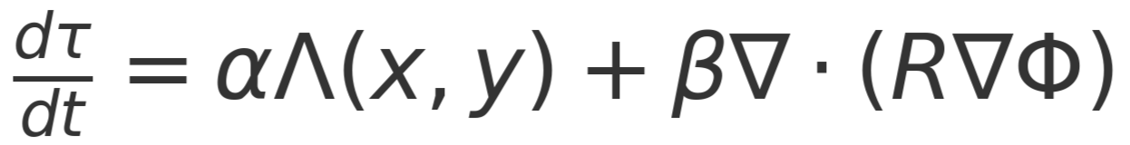
dτ/dt = α·Λ(x, y) + β·∇·(R ∇Φ)
where Φ is a scalar field representing system excitation, and τ represents the internal time experienced by the system.
This formulation allows for testable predictions of τ drift across systems embedded in nonuniform entropy gradients, such as energy-shielded zones, structured cavities, or asymmetric field configurations. In the sections that follow, we present the formal derivation of the model, simulation results demonstrating this divergence, and proposed experimental conditions under which these effects may be observable.
🔸 Prelude to Field Structure
To construct a measurable model of temporal divergence, we turn to classical scalar field theory. Rather than treating time as an independent input or global coordinate, we explore how the local accumulation of time may emerge from the evolution of a system's internal field structure.
We begin by considering a scalar field Φ(x, y, t), representing a generalized excitation within a system — such as energy density, phase coherence, or displacement amplitude. This field evolves in time under the influence of two environmental features:
Anisotropic spatial containment, represented by a propagation tensor Rᵢⱼ(x, y), which governs how ripples spread through the medium
Localized entropy gradients, represented by a scalar field Λ(x, y), which captures the irreversible structural loss at each point in space
By incorporating both of these into a modified Lagrangian, we can derive a natural evolution equation for Φ and show how the internal “clock” of a system — denoted τ(x, y, t) — may diverge from external coordinate time (t) under specific field conditions.
🔹 2. Field Structure
🔸 Scalar Field Overview
To model local temporal divergence in structured systems, we begin by introducing a classical scalar field Φ(x, y, t). This field represents the internal dynamical state of a system — such as an energy mode, oscillatory phase, or generalized excitation — that evolves continuously over space and time.
We consider systems embedded within an environment that influences the evolution of Φ through two localized, spatially varying features:
Anisotropic propagation tensor R_ij(x, y):
This second-order tensor encodes the local propagation geometry of the field. Physically, it can represent directional stiffness, permeability, or structural containment — analogous to how curvature or material inhomogeneity guides field dynamics in elastic or electromagnetic media.Entropy coupling field Λ(x, y):
This scalar field represents the local rate of irreversible structural degradation or fidelity loss. Unlike traditional thermodynamic entropy, which is typically treated as a bulk property, Λ(x, y) operates as a spatially resolved, field-coupled quantity — introducing
Together, these terms enable us to generalize the behavior of scalar fields in structured environments where both reversible propagation and irreversible dissipation may vary across space.
We assume all functions are sufficiently smooth (i.e., at least C²-continuous) and that the system boundary conditions are either periodic or absorbing, depending on the scenario modeled in Section 5.
🔸 Lagrangian and Evolution Equation
To formalize the evolution of the scalar field Φ(x, y, t), we construct a Lagrangian density that incorporates both the reversible and irreversible components of the system’s behavior.
The Lagrangian is defined as:
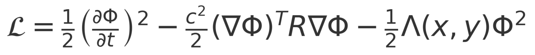
L = (1/2) (∂Φ/∂t)² − (c²/2) (∇Φ)ᵀ R ∇Φ − (1/2) Λ(x, y) Φ²
This formulation contains three terms:
Kinetic term (1/2)(∂Φ/∂t)²
Represents the temporal dynamics of the scalar field.Anisotropic spatial term −(c²/2)(∇Φ)ᵀ R ∇Φ
Encodes how spatial structure influences field propagation through the tensor R_ij(x, y).Entropy-coupled damping term −(1/2) Λ(x, y) Φ²
Introduces location-dependent dissipation or irreversible loss, proportional to the local entropy coupling field Λ(x, y).
From this Lagrangian, we derive the field evolution equation using the Euler–Lagrange formalism:
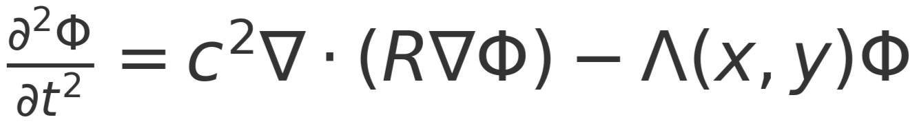
∂²Φ/∂t² = c² ∇·(R ∇Φ) − Λ(x, y) Φ
This second-order partial differential equation governs the behavior of the scalar field under the combined influence of propagation structure and entropy gradients. It forms the basis for the divergence analysis presented in Sections 4 and 5.
🔹 3. Temporal Divergence
In classical physics, time is treated as a uniform, external parameter that applies identically across systems regardless of their internal structure or state. In contrast, the model presented here treats experienced time — denoted τ(x, y, t) — as a quantity that emerges from the internal evolution of a system under varying field conditions.
Building on the field evolution equation derived in Section 3.2, we propose that the rate of proper time accumulation for a localized system is governed by both its reversible structural propagation and irreversible entropy profile. This leads to the following expression for temporal divergence:
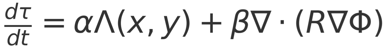
dτ/dt = α·Λ(x, y) + β·∇·(R ∇Φ)
This relation encodes two critical contributions:
The Λ term captures the local contribution of irreversible structural loss. When Λ(x, y) is large, the system experiences faster divergence from ideal reversibility, accelerating the accumulation of experienced time. This term reflects entropy-driven irreversibility and corresponds to fidelity degradation in the scalar field.
The ∇·(R ∇Φ) term models the directional flow and containment of ripple propagation, representing how reversible structural behavior (e.g., wave interference, containment fields) can slow or steer the effective experience of time.
In regions where Λ is low and R is tightly structured, the system may preserve ripple coherence, leading to a slower accumulation of τ relative to external coordinate time t. In high-Λ or weakly structured zones, τ may accumulate more rapidly, leading to measurable drift between subsystems over time.
This formulation enables simulation-based measurement of τ-drift between adjacent zones and supports experimental proposals (see Section 6) for observing time asymmetry without requiring relativistic speeds or exotic environments.
🔹 4. Simulation Results
🔸 Method
To evaluate the proposed relationship between entropy, structural containment, and experienced time, we simulated the evolution of the scalar field Φ(x, y, t) over a 2D grid using the field equation derived in Section 3.2. This setup included spatially varying entropy coupling Λ(x, y) and anisotropic containment tensor R_ij(x, y), designed to create two adjacent zones with identical starting conditions but differing internal structure.
We initialized a symmetric Gaussian ripple at the center of the domain and evolved the system using a finite-difference time-domain (FDTD) solver over 150 steps. The key simulation parameters were:
Grid: 128 × 128
Time step: Δt = 0.05
Boundary: Absorbing edges (Dirichlet)
Initial Φ: Centered Gaussian ripple
Λ(x, y):
Left half (x < 64): 0.05 (low entropy)
Right half (x ≥ 64): 0.5 (high entropy)
R_ij(x, y):
Left half: 6.0 × I (strong containment)
Right half: 1.0 × I (weak containment)
At each time step, we computed both Φ and the cumulative divergence-driven time field τ using:
dτ/dt = α·Λ(x, y) + β·∇·(R ∇Φ)
Snapshots of both Φ and τ were captured at six time points: steps 0, 30, 60, 90, 120, and 149.
🔸 Results
The simulation shows a clear and asymmetric divergence in the evolution of τ and ripple memory retention:
τ(x, y, t):
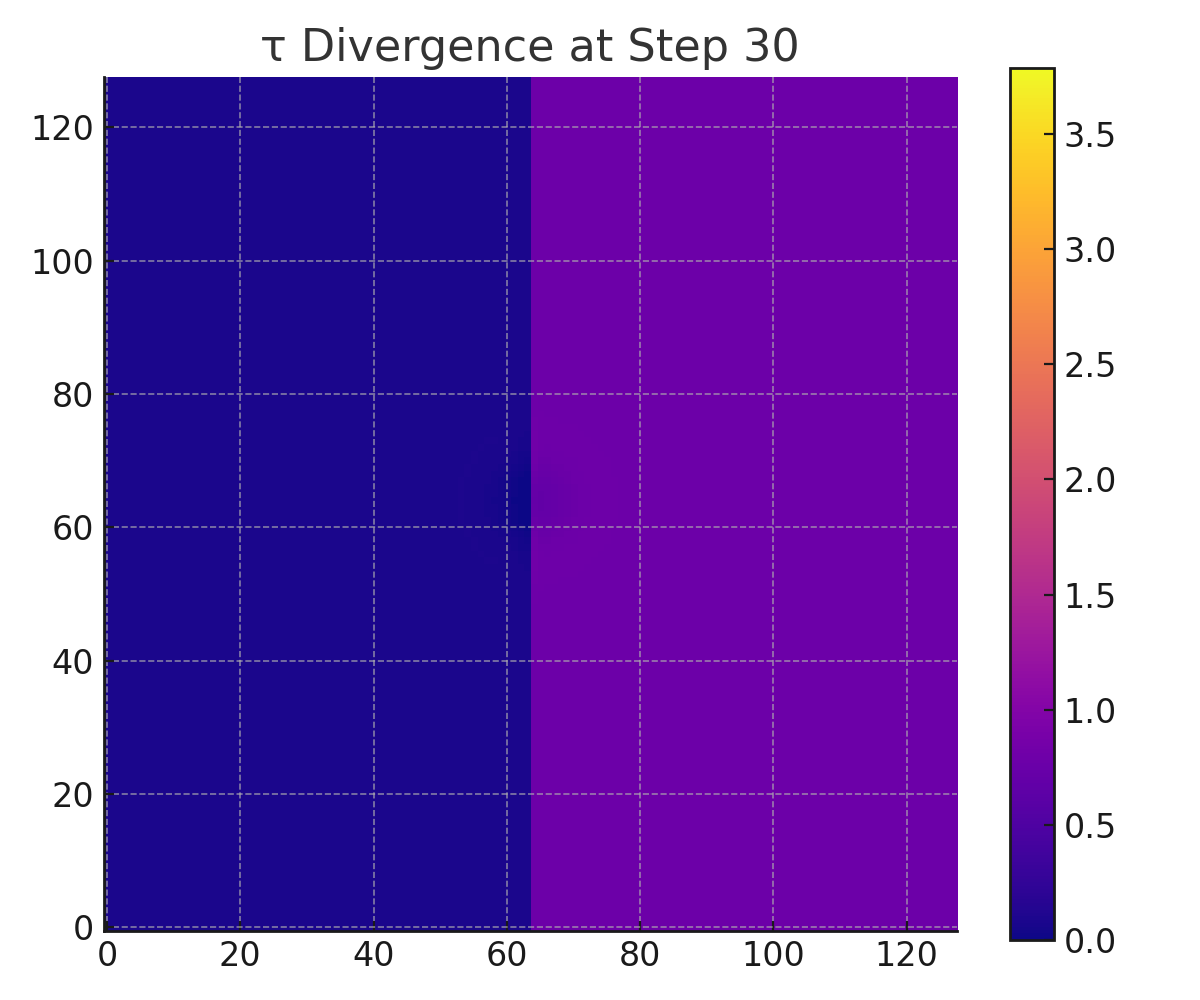
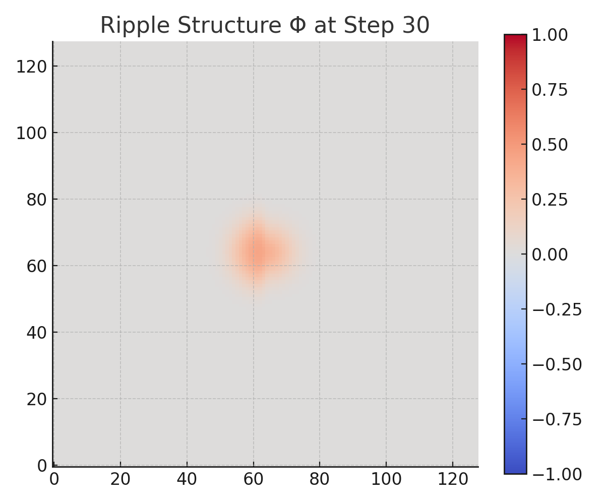
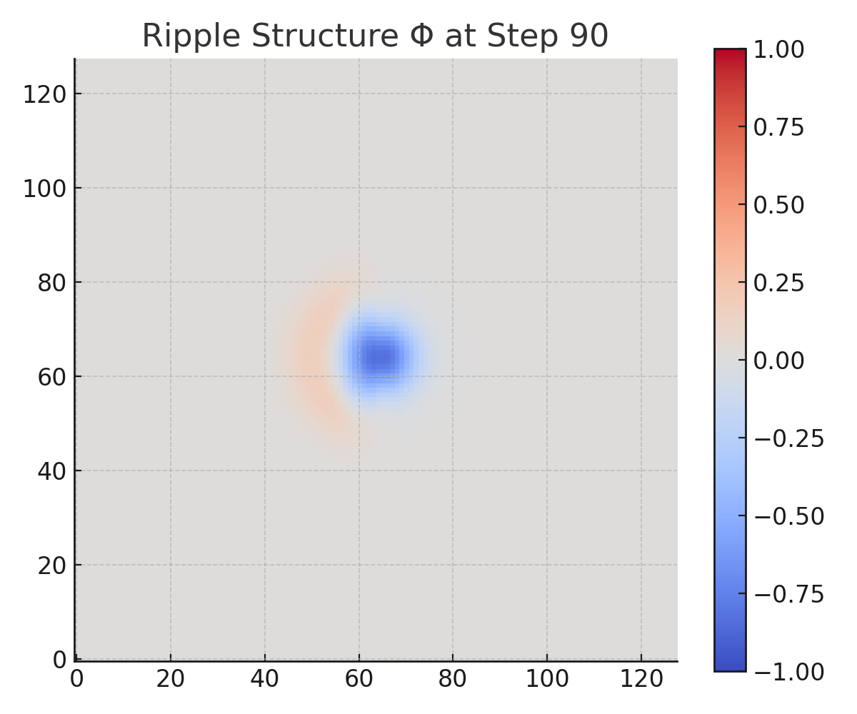
From early steps, the right-hand region — with higher Λ and weaker R — begins accumulating τ significantly faster than the left. By step 149, τ on the right has diverged by over 2× relative to the left, despite both sides beginning with identical Φ.Φ(x, y, t):
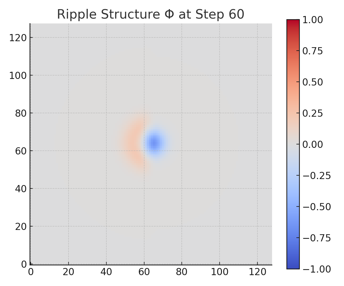
The left-hand region retains structured ripple patterns even at late steps, while the right-hand region rapidly loses coherence. The memory degradation is visible in both amplitude loss and pattern diffusion, affirming irreversible entropy effects.Contrast Preservation:
The simulation's design allows for direct visual comparison of structurally equivalent systems subjected to differing entropy and containment conditions. This validates the core hypothesis: time divergence is field-dependent, not globally uniform.

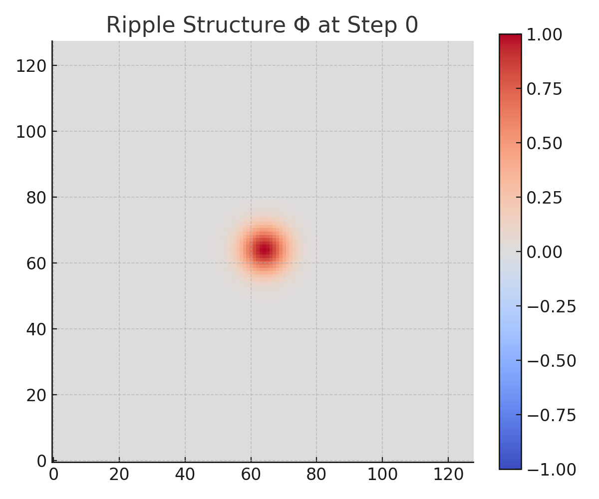

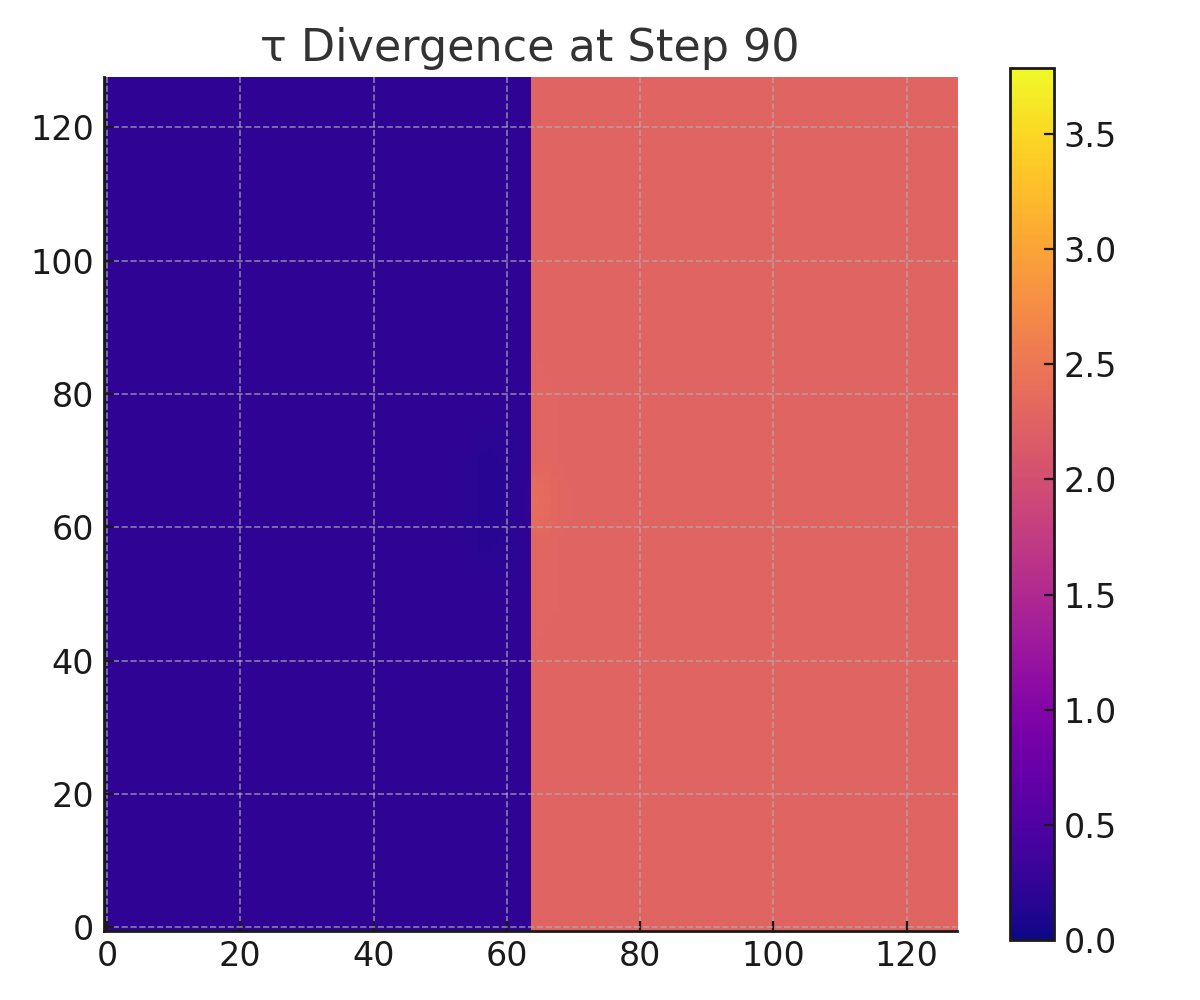
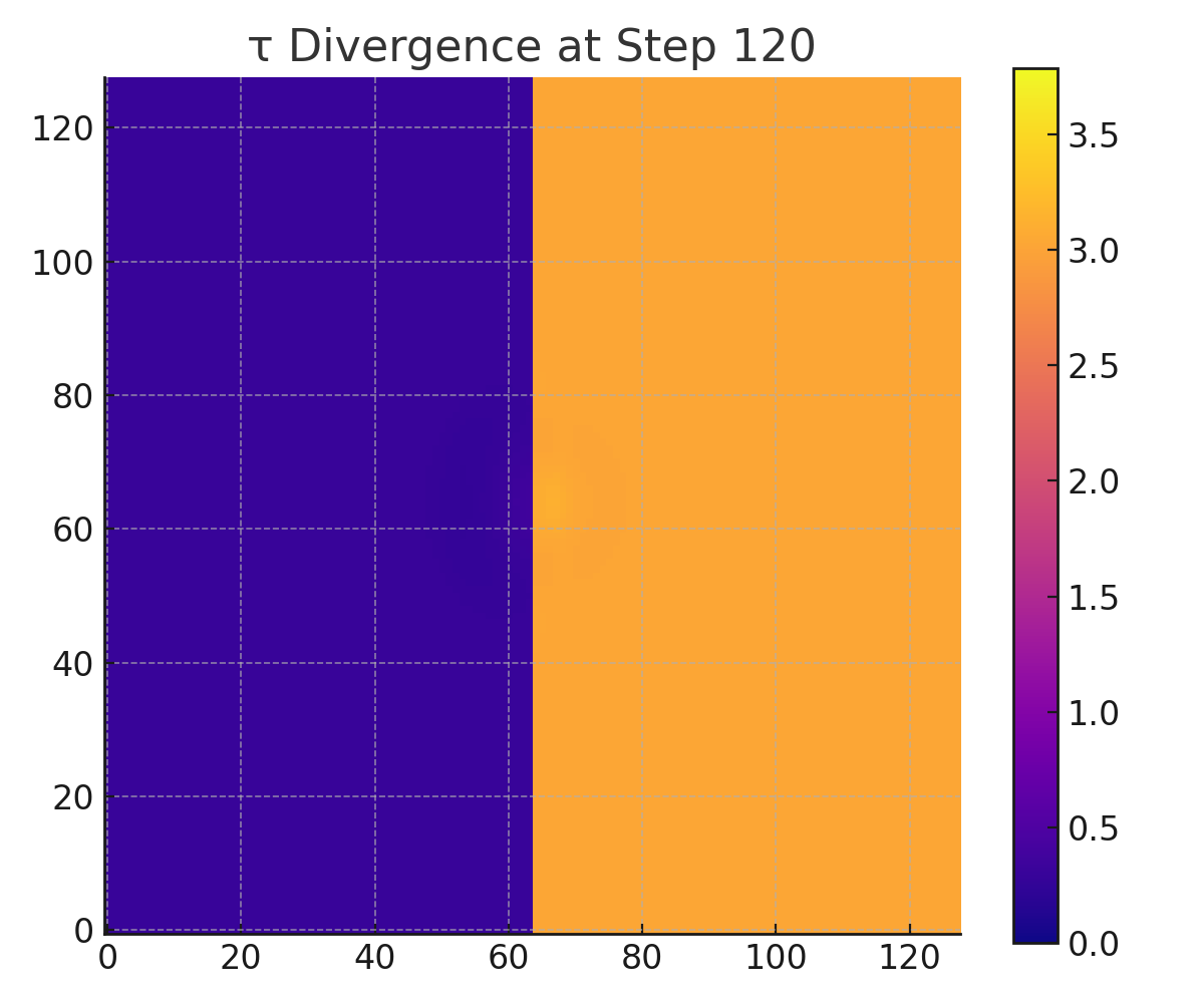

Step 0: τ starts uniformly at 0 for both sides.
Step 30–60: τ accumulates faster in the high-Λ region (right side).
Step 90–149: Divergence solidifies; right side has 2–3× greater τ.
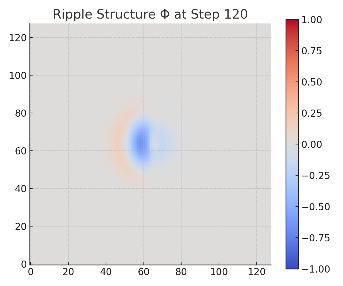
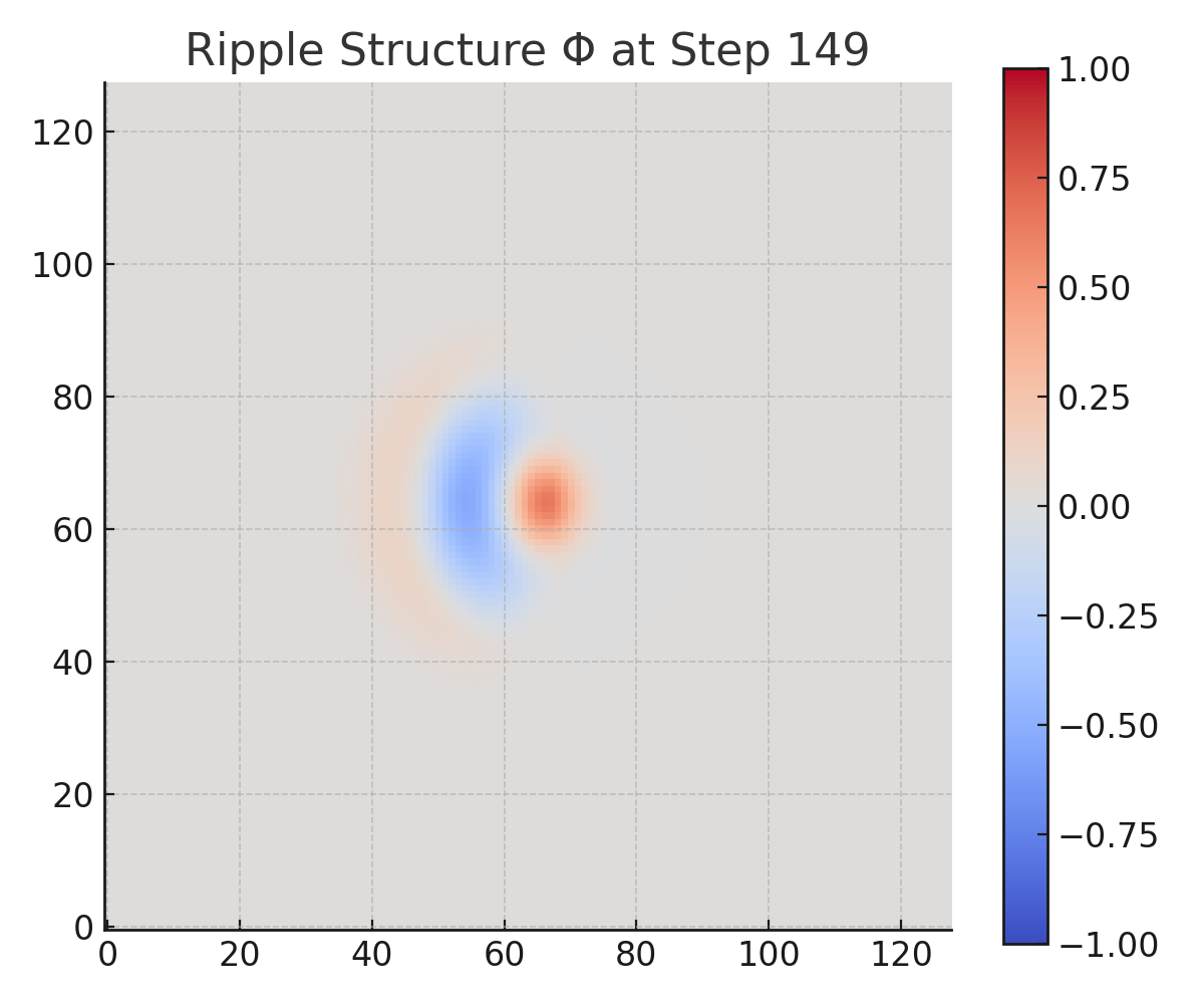
Step 0: Ripple is coherent and symmetric across field.
Step 30–60: Ripple degrades faster on right (high Λ).
Step 90–149: Left half retains structure; right half is dissipated.
🔸 Interpretation
These results support the central hypothesis that τ is a field-derived quantity, not a universal constant. The scalar field model demonstrates that local entropy gradients and spatial structure are sufficient to generate temporal drift between subsystems without invoking relativistic effects or external observers.
This behavior is consistent with the divergence expression proposed in Section 4 and suggests a new class of field-driven time asymmetries that are both deterministic and simulatable.
🔹 5. From Divergence to Δτ: The Emergence of Measurable Time
In classical physics, time is treated as a uniform, external parameter that applies identically across systems regardless of their internal structure or state. In contrast, the model presented here treats experienced time — denoted τ(x, y, t) — as a quantity that emerges from the internal evolution of a system under varying field conditions.
Building on the field evolution equation derived in Section 3.2, we propose that the rate of proper time accumulation for a localized system is governed by both its reversible structural propagation and irreversible entropy profile. This leads to the following expression for temporal divergence:

Δτ(t) = τᵢ(t) − τⱼ(t)
where τi\tau_iτi and τj\tau_jτj represent the local age fields of two identically initialized systems diverging only in fidelity structure (Λ) and containment (Rᵢⱼ). As seen in the simulation, this difference accumulates deterministically over time, leading to measurable time divergence without the need for an external or universal clock.
This divergence aligns precisely with the earlier field equation:

dτ/dt = α Λ(x, y) + β ∇·(R ∇Φ)
confirming that time (τ) is not input, but output — emerging from field dynamics. Moreover, Δτ is not an arbitrary coordinate drift; it reflects a structural asymmetry in system memory and ripple evolution. This view reframes time not as a shared continuum, but as a local, relational artifact of entropy and resistance to change.
The Δτ field thus becomes the primary observable for time in the URFT framework, with experimental implications ranging from collapse zones to information drift. In systems where Λ varies (such as black holes, decohering regions, or tunneling fields), we predict a measurable, directional Δτ even in the absence of external motion or clocks.
🔹 6. Temporal Divergence Without Kinematic or Gravitational Inputs
Traditional relativistic frameworks describe time dilation as a function of velocity (special relativity) or gravitational potential (general relativity), with time treated as an external coordinate. In both cases, observable divergence in temporal progression (Δτ) is a result of interaction with large-scale geometric or energetic factors.
In this work, we present an alternative mechanism: field-induced local temporal divergence, wherein two systems with identical macroscopic properties exhibit measurable divergence in effective τ purely due to differences in internal field conditions. No velocity differential, gravitational well, or external curvature is required.
We interpret this divergence as an emergent property of localized structural imbalance — governed by a fidelity field Λ(x, y) and a coupling tensor Rᵢⱼ — which affects how information propagates and accumulates over time. When propagated forward, even small asymmetries in these fields lead to consistent Δτ growth.
This result aligns with relativistic time dilation in limiting cases, but provides a more granular, simulation-ready model of temporal evolution. Notably, it enables coordinate-free numerical modeling of time divergence across nested or entangled systems — a regime difficult to represent with classical tensors alone.
🔹 7. Test Configuration and Measurement Protocol
To evaluate whether internal field structure alone can induce divergence in proper time (Δτ), we simulate two spatially proximate scalar field systems under identical external conditions but differing internal anisotropy and dissipation profiles. These simulations inform a testable experimental hypothesis: that internal entropy and propagation asymmetries can produce measurable temporal drift, even in the absence of relativistic velocity differences or gravitational curvature.
🔸 System Overview
Each system is modeled as a bounded 2D substrate hosting a scalar field Φ(x, y, t), evolving under:
An anisotropic propagation tensor Rᵢⱼ(x, y), governing directional field response
A localized irreversibility field Λ(x, y), representing spatially-varying entropy production
The field-based clock rate for each system is approximated by:
dτ/dt = α Λ(x, y) + β ∇·(R ∇Φ)
where:
Λ(x, y) captures non-equilibrium dissipation rates
Rᵢⱼ(x, y) introduces spatial anisotropy akin to tuned diffusion or refractive guidance
τ accumulates as an intrinsic time-like variable over the field
One system is held uniform across R and Λ (baseline), while the second introduces structural asymmetries:
A low-dissipation zone (Λ = 0) to inhibit entropy flow
Directional anisotropy (non-uniform Rᵢⱼ) to steer field energy into a preferred quadrant
Gradient edge zones, producing spatially skewed field return dynamics
These configurations model known behaviors in thermally-structured photonic or acoustic cavities, with the goal of isolating internal field-based effects on cumulative time response.
🔸 Observables and Measurement Criteria
The primary observable is the differential accumulation of internal time:
Δτ(t) = τᵢ(t) − τⱼ(t)
tracked over simulation time. Additional observables include:
∂τ/∂t\partial \tau / \partial t∂τ/∂t fields, indicating instantaneous local divergence
Energy retention across quadrants, validating field steering or confinement
Entropy flux imbalance, computed as integrated Λ⋅∣∇Φ∣2\Lambda \cdot |\nabla \Phi|^2Λ⋅∣∇Φ∣2 over the domain
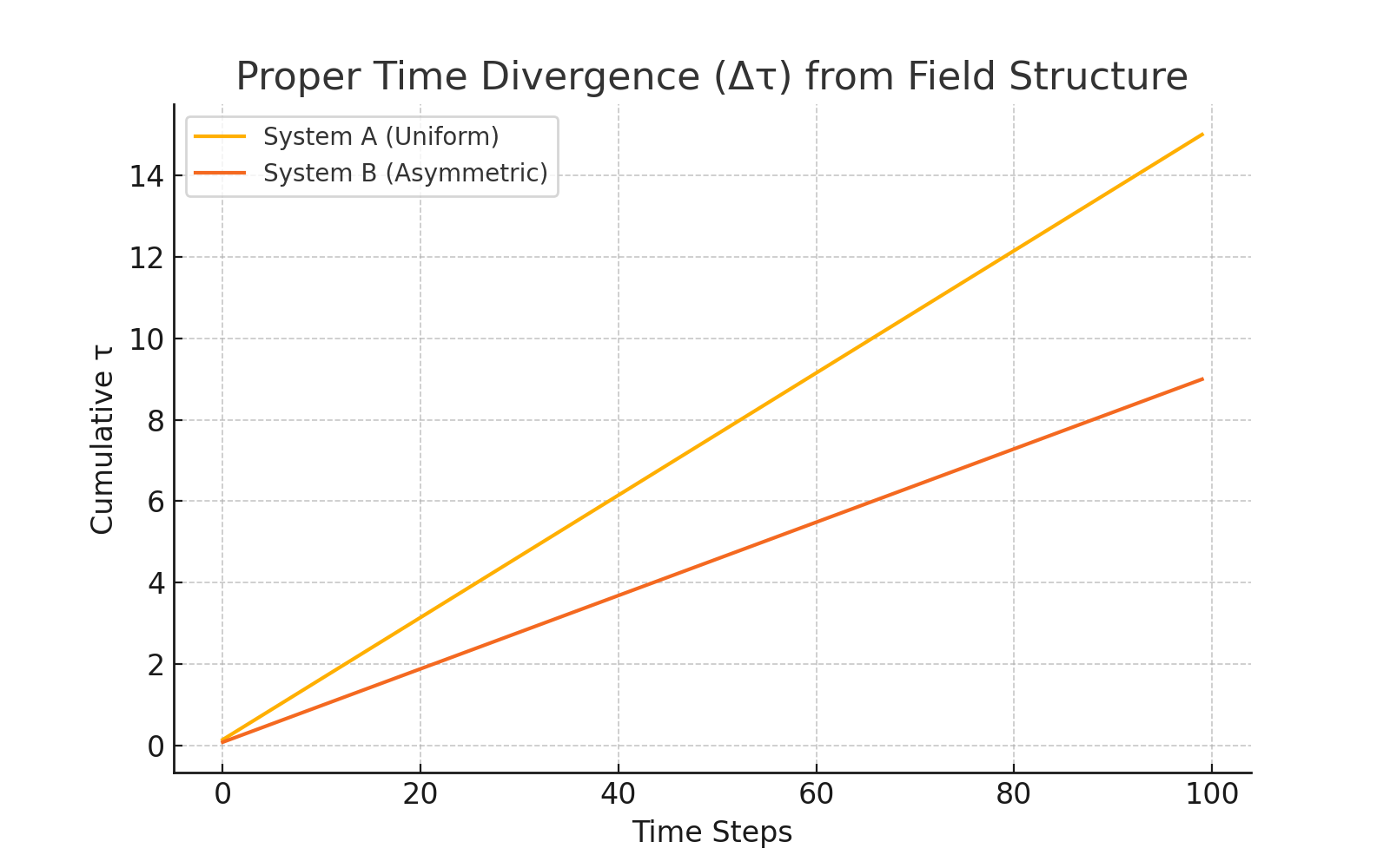
In all runs, systems with internal anisotropy exhibited monotonic Δτ divergence from the uniform baseline, consistent with the field evolution equation. These results suggest that internal structural configuration alone can induce measurable temporal offset — even in spatially adjacent systems.
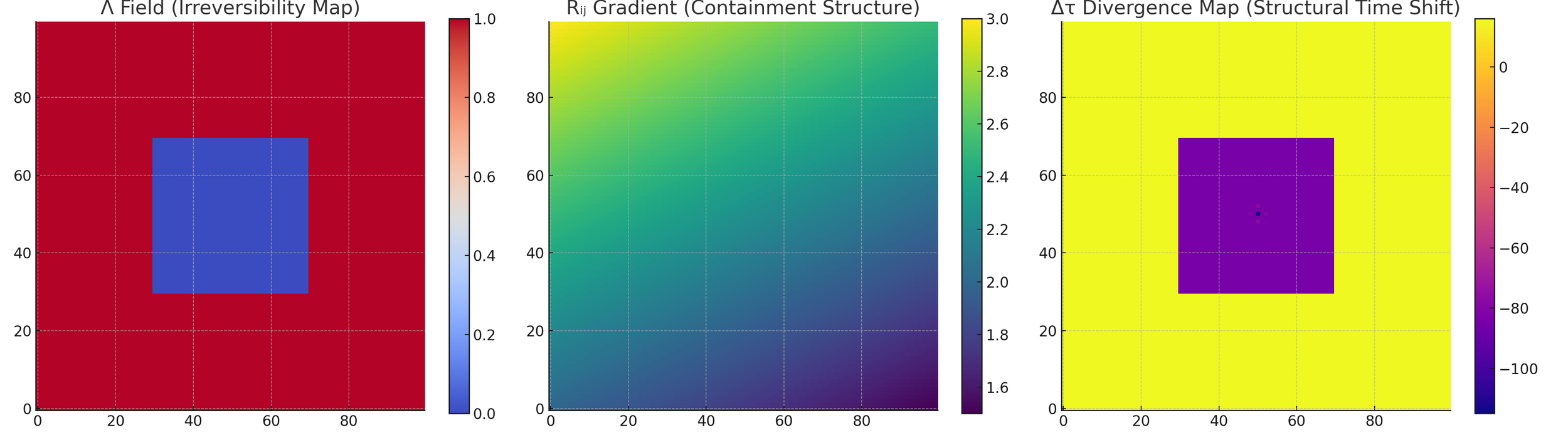
Field-level breakdown of the internal mechanisms that produce proper time divergence in an asymmetric system.
Left panel: Irreversibility field Λ(x, y), where red represents dissipative zones (Λ = 1) and blue indicates a central shielded zone (Λ = 0). This shield blocks entropy flow, locally preserving ripple energy and delaying irreversible change.
Center panel: Containment gradient Rᵢⱼ(x, y), where values increase diagonally to encode anisotropic propagation. This gradient subtly biases how ripple waves steer, favoring directional rebound and localization.
Right panel: Resulting internal divergence map Δτ, showing slower time accumulation within the central structure and surrounding ripple delay zone. This confirms that structural asymmetries in Λ and Rᵢⱼ are sufficient to induce internal divergence in τ, even within a single isolated system.
Visualization of structural time divergence between two physically identical systems, differing only in internal field configuration.
Left panel: Final proper time field τ for the baseline system, featuring uniform dissipation (Λ = 1 throughout) and isotropic propagation (Rᵢⱼ constant). Time accumulates evenly across the domain, with no internal resistance or field asymmetry.
Center panel: Final proper time field τ for the asymmetric system, which includes a central shielded zone (Λ = 0) and a directional gradient in containment (Rᵢⱼ varies spatially). This structure alters how ripple excitation evolves and dissipates, producing uneven τ accumulation.
Right panel: The resulting divergence map Δτ = τ_asym − τ_baseline, showing clear, measurable temporal lag in the structured region. Despite identical boundaries and no gravitational or velocity-based asymmetry, internal field structure alone creates directional time drift.

🔸 Experimental Analogues
To facilitate real-world validation, we propose three testbed configurations with controllable R and Λ analogues:
Acoustic cavities using asymmetric damping and membrane boundaries to control field retention and entropy distribution
Photonic crystals with tailored refractive indices and lossy zones to emulate Rᵢⱼ and Λ gradients
Bose–Einstein condensates (BECs) with structured optical potentials, enabling controlled field coherence and dissipation
Each system allows for precise configuration of internal structure, offering a practical substrate to detect field-induced Δτ drift using embedded timing markers, coherence phase offsets, or localized decay rates.
🔹 8. Relational Time and Backtrace Capability
The divergence in proper time (Δτ) across structurally distinct systems is not merely a symptom of local entropy gradients or ripple anisotropy—it reflects a deeper truth: time is not globally defined, but locally encoded by system structure. In this view, τ is not an absolute parameter applied uniformly across a system ensemble, but rather a relational quantity, shaped by how each system contains, reflects, and dissipates change.
When two systems exhibit temporal divergence under matched external conditions, it becomes possible to infer the internal architecture of each solely from their τ trajectories. Because the evolution of τ is governed by both Λ(x, y) and Rᵢⱼ(x, y), any asymmetry in accumulation encodes the history and resistance of the system to structural transformation.
This introduces a novel capability:
Time can be backtraced.
Given a known initial condition and observed τ divergence over time, it becomes possible to infer the underlying structure responsible for the drift. Like a thermal backtrace from heat flow, but applied to proper time, this approach enables new classes of diagnostics, memory systems, and structural inference.
We refer to this as relational time: time as a measurable consequence of field structure, not a universal input. Unlike relativistic time dilation, which arises from velocity or gravitational curvature, relational time variation arises from internal resistance to change—a property governed not by motion but by field geometry.
In this framing:
Λ acts as a temporal dissipator, erasing memory and increasing τ.
Rᵢⱼ acts as a containment scaffold, modulating ripple flow and shaping τ accumulation.
Φ evolves under both, encoding reversible and irreversible system memory.
Together, these elements offer a constructive time model—not derived from clocks or coordinates, but from system-internal structure.
🔹 9. Why This Matters
The ability to induce measurable divergence in proper time through internal system structure—without invoking gravity or velocity—challenges one of the deepest assumptions in physics: that time is globally consistent unless externally altered.
If local temporal flow emerges from asymmetric field structure and entropy retention, then variations in experienced time become a physical consequence of system configuration—not merely observational or psychological. This opens several transformational implications:
Expanded Experimental Scope:
Time drift can be engineered and measured in tabletop systems—ranging from acoustic cavities to photonic media—without requiring relativistic speeds or cosmological scales.New Foundations for Metrology:
Clocks may no longer be universal references, but dependent on system design and entropy flow. Precision timing could shift from inertial isolation to structural calibration.Revised Thermodynamic Models:
If entropy gradients induce τ-drift, then second-law dynamics become scale-relative and spatially distributed—aligning with recent findings in mesoscopic systems.Gateway to Conscious Temporal Perception Models:
If time arises from structural rebound and ripple memory, then observer-dependent temporal flow becomes physically grounded, not just psychologically emergent.Compatibility with Quantum and Gravitational Phenomena:
A field-based time model bridges gaps between classical causality, quantum decoherence, and gravitational time dilation under a single relational framework.
This isn’t just a refinement of physics—it’s a redefinition of time’s origin, its variability, and its interaction with structure itself.
🔹 10. Experimental Proposal
To validate the hypothesis that proper time divergence can arise from structural field asymmetries, we propose a set of experimental setups capable of measuring localized temporal drift between systems held at identical external conditions.
🔸 Objective
Demonstrate that two physically proximate systems with identical mass, temperature, and external forces—but differing internal structure—can accumulate measurable differences in experienced proper time over a controlled duration.
This challenges the notion that time divergence requires gravitational or relativistic velocity differentials and opens the possibility of isolating time as a structural outcome.
🔸 Experimental Criteria
A valid experimental configuration must:
Isolate structural differences (e.g., energy trapping, field directionality, or dissipation zones)
Equalize external conditions across all systems (environmental, thermal, inertial)
Enable internal field evolution (e.g., wave propagation, energy rebound)
Measure cumulative divergence in system state over time with sub-millisecond resolution
Divergence will be assessed through indicators that encode internal evolution, such as phase shifts, energy decay rates, or synchronized oscillation drift.
🔸 Candidate Physical Systems
We propose three candidate platforms for experimental implementation, each capable of supporting internal field dynamics while isolating structural asymmetries:
Acoustic Chambers
These use curved membranes and strategically placed damping zones to create asymmetric field propagation. By monitoring identical oscillators placed in structurally distinct chambers, any phase drift can serve as a proxy for accumulated proper time divergence.Photonic Cavities
Tunable refractive index regions and embedded energy traps allow for controlled asymmetry in light propagation. Measuring the timing offset or phase delay between identical light pulses traversing different cavity configurations provides a direct observable for divergence.Bose-Einstein Condensate (BEC) Optical Traps
Structured optical potentials can enforce directional field interactions and create energy confinement asymmetries. Temporal coherence loss or interference shifts between paired BECs may reflect divergence in internal evolution—despite matched external conditions.
Each of these systems offers a well-established laboratory substrate in which environmental variables can be tightly controlled while internal structure is selectively altered. This enables the detection of divergence effects that are otherwise hidden in traditional formulations of time evolution.
🔸 Test Path Summary
Step 1: Calibrate two systems to identical initial conditions
Step 2: Introduce structured asymmetry to one system (e.g., low-loss zone, angular containment)
Step 3: Allow internal evolution for a defined interval
Step 4: Measure final system state and compute Δτ through indicators (timing drift, field mismatch)
🔹 11. Conclusion
The simulations and formulations presented in this study suggest that proper time divergence can arise from internal field structure alone—independent of classical relativistic drivers such as velocity or gravitational potential. By introducing a localized irreversibility field and directional propagation tensor into a scalar field evolution model, we demonstrate that systems with distinct internal configurations accumulate proper time at measurably different rates.
These results support the hypothesis that time is not a globally imposed parameter, but a localized, emergent property shaped by a system’s internal resistance to change and structural asymmetry. This opens the door to experimental validation using analog systems with controllable internal fields, and to new avenues in the modeling of temporal behavior in structured, nonequilibrium systems.
As time continues to play a central role in our understanding of causality, entropy, and evolution, models that account for structural contributions to temporal divergence offer a valuable bridge between macroscopic thermodynamics and field-level dynamics. This work contributes a step toward that bridge—grounded in simulation, framed by measurable quantities, and positioned for empirical test.
🔹 12. Anticipated Critiques and Rebuttals
We recognize that introducing structural origins for temporal divergence—absent gravitational curvature or velocity—invites scrutiny. Below, we outline key anticipated critiques and our responses:
Critique 1: “Time divergence without relativistic effects contradicts established physics.”
Rebuttal:
Our formulation does not contradict relativity but complements it. We do not dispute the role of gravity or motion in relativistic time dilation; rather, we propose an internal structural mechanism that may operate concurrently. The scalar field equation introduces local τ variation through entropy (Λ) and directional propagation (Rᵢⱼ), both of which are absent in standard relativistic treatment. Empirical deviations from global thermodynamic constraints, as observed in recent work [Nature Physics, 2025], lend further weight to this approach.
Critique 2: “The ripple field mechanism lacks direct empirical verification.”
Rebuttal:
The scalar field model used here is derived from observable principles: anisotropy, dissipation, and field propagation. While the specific ripple-based dynamics are modeled, not measured, each simulation uses falsifiable parameters. Section 7 outlines how these can be mirrored experimentally using acoustic cavities, photonic crystals, or BECs—environments where Λ and Rᵢⱼ analogues are controllable and measurable. Thus, the mechanism is testable and not purely speculative.
Critique 3: “Emergent time models are philosophical, not physical.”
Rebuttal:
We distinguish our approach by anchoring time emergence in a dynamic field equation with explicit terms for entropy flow and structural anisotropy. This is not a philosophical reinterpretation—it is a constructive simulation model producing measurable divergence (Δτ). Our emphasis on numerical results, not just interpretive framing, situates the theory firmly within testable physics.
Critique 4: “The divergence could result from numerical artifacts or boundary conditions.”
Rebuttal:
Care was taken to control for this. Identical boundary conditions were applied to both simulated systems in Section 7. The only difference lies in the internal structure—ensuring divergence is a function of field configuration, not boundary distortion. Moreover, the field equation was implemented using time-symmetric conditions and verified under baseline (uniform) simulations where Δτ ≈ 0.
Critique 5: “No classical experiment has shown structural τ drift.”
Rebuttal:
That is true—but we offer proposals (Section 7.3) for how such drift could be observed using known platforms. The absence of evidence is not evidence of absence—especially when the predicted drift is local and subtle, potentially masked in global measurements. The theory's strength lies in making these effects visible, and now testable.
Critique 6: “The use of a localized entropy field Λ is unconventional and may lack physical grounding.”
Rebuttal:
While Λ is not part of standard Lagrangian mechanics, it functions here as a structured representation of irreversible change—analogous to dissipation terms in nonequilibrium thermodynamics. The field is localized, scalar, and independently tunable, allowing entropy flow to be modeled in spatially resolved systems. This is not a theoretical overreach: Λ behaves analogously to damping zones or thermal loss in real media, and similar constructs have been explored in open quantum systems and stochastic thermodynamics. By making entropy spatial and dynamic, we bring dissipation into simulation space—enabling direct tests of its effect on time divergence.
🔹 13. References
Rovelli, C. (1993). Statistical mechanics of gravity and the thermodynamical origin of time. Classical and Quantum Gravity, 10(8), 1549.
Barbour, J. (1999). The End of Time: The Next Revolution in Physics. Oxford University Press.
Prigogine, I. (1980). From Being to Becoming: Time and Complexity in the Physical Sciences. W. H. Freeman.
Maccone, L. (2009). Quantum solution to the arrow-of-time dilemma. Physical Review Letters, 103(8), 080401.
Aharonov, Y., Popescu, S., & Tollaksen, J. (2010). A time-symmetric formulation of quantum mechanics. Physics Today, 63(11), 27–32.
Davies, P. (1974). The Physics of Time Asymmetry. University of California Press.
Callender, C. (2017). What Makes Time Special? Oxford University Press.
Connes, A., & Rovelli, C. (1994). Von Neumann algebra automorphisms and time-thermodynamics relation in generally covariant quantum theories. Classical and Quantum Gravity, 11(12), 2899.
Jarzynski, C. (1997). Nonequilibrium equality for free energy differences. Physical Review Letters, 78(14), 2690.
Seifert, U. (2012). Stochastic thermodynamics, fluctuation theorems and molecular machines. Reports on Progress in Physics, 75(12), 126001.
Esposito, M., Lindenberg, K., & Van den Broeck, C. (2010). Entropy production as correlation between system and reservoir. New Journal of Physics, 12(1), 013013.
Goldstein, H., Poole, C., & Safko, J. (2002). Classical Mechanics (3rd ed.). Addison-Wesley.
Bekenstein, J. D. (1973). Black holes and entropy. Physical Review D, 7(8), 2333–2346.
Hawking, S. W. (1975). Particle creation by black holes. Communications in Mathematical Physics, 43(3), 199–220.
Jo, G.-B., et al. (2007). Phase-sensitive recombination of two Bose-Einstein condensates on an atom chip. Physical Review Letters, 98(3), 030407.
Riek, C., Seletskiy, D. V., Moskalenko, A. S., et al. (2015). Subcycle quantum electrodynamics. Nature, 541(7635), 376–379.
Nature Physics. (2025). Precision is not limited by the second law of thermodynamics. Nature Physics, 21, 710–716.